Optimizing Mixed Refrigerant Composition
Joel Cantrell
January 25, 2017
Liquefying natural gas efficiently requires complex design, complex operation, or both. The process must cool, condense, and subcool a multicomponent mixture across an enormous temperature range. In the case of the classical cascade refrigeration, the refrigerants are relatively simple, but the multiple interconnected refrigeration loops are not. With a mixed refrigerant system, the roles are reversed. The equipment is relatively simple, as shown in Figure 1, but the complexity has been moved to the refrigerant mixture.
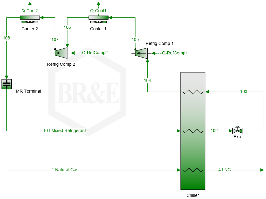
Figure 1 – Single Mixed Refrigerant System
As a further comparison, the classical cascade system has a finite number of discrete cooling temperature steps while the mixed refrigerant system has a continuous cooling curve due to a boiling mixture through most of the process. Figure 2 shows the supply and demand curve for a single mixed refrigerant system. This example process is an exercise from the BR&E training course BRE 202 LNG Processing.

Figure 2 – SMR Cooling Curve
The temperature difference between the supply and demand curves represents heat transfer inefficiency. One of the major factors in the shape of this curve is the composition of the refrigerant. As such, the composition becomes an optimization variable for increasing energy efficiency. One technique for optimizing the composition is through the use of the ScenarioTool® in ProMax®. The changes in the composition are selected by the user. The results are then displayed and observations can be made regarding the effectiveness and sensitivity of the changes. Table 1 shows the outcome of several ScenarioTool cases. Increasing the nitrogen and n-butane at the expense of methane improved performance notably. While it does give the user a sense of the direction needed to improve the performance, it does not provide a single optimal answer.

Table 1 – ScenarioTool results
A second possibility for optimization is the Excel Solver. The spreadsheet information and solver dialog needed to drive the optimization is shown in Figure 3. The objective function to be minimized is the total of the refrigerant compressor power. In this application, the ethane through nitrogen compositions are varied and the methane composition is calculated by difference. The optimizer could calculate a composition that essentially sets the two cooling curves on top of one another or allow a negative approach, giving an impossible heat transfer situation. To keep the system rational, a minimum effective approach temperature (MEAT) of 2°C was imposed. This becomes a constraint to the system.
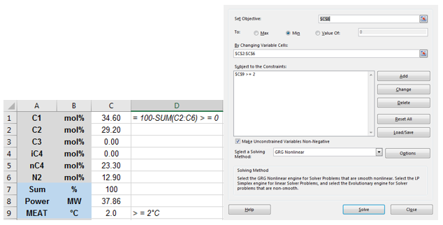
Figure 3 Excel Solver parameters
In addition to the Excel input, some VBA code is necessary to trigger the ProMax solve for a composition input.
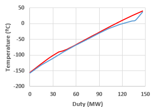
Figure 4: Optimal cooling curve
Figure 4 shows the result of the optimization. The supply and demand curves are very close together. The best case found ‘by hand’ was 38.8 MW, while the optimizer went further and located a mixture that gave 37.9 MW.
It should be noted that the optimal composition is dependent on all the other factors in the process, including natural gas inlet pressure, temperature and composition, refrigerant pressure and temperature, compressor efficiency, and heat exchanger temperature approach. Because of this, while the optimal target is good to know, the sensitivity of this optimal target to the external conditions would be important as well. This is shown in Table 2 for variations from the base natural gas pressure of 36 bar. Note that the composition remains the same for the changing conditions. The higher the gas pressure, the easier the liquefaction. However, the solution at 36 bar was at the approach temperature constraint of 2ºC. When the pressure dropped below the nominal value, the constraint would be violated, even at a higher energy usage.

Table 2: Sensitivity to feed pressure
The optimization routine could be repeated for the two pressure variations. However, if these variations are transient or changing the refrigerant blend is difficult, the sensitivity of the nominal mixture must be considered.
There are other potential optimization variables for a mixed refrigerant system, such as feed pressure and refrigerant expansion pressure, that could be addressed in future optimization projects. Please contact BR&E Support if you would like additional information on this procedure.